
Deriving temperatures from RMR lidar measurements
Whenever permitted by the weather, the IAP RMR lidar and the ALOMAR RMR lidar are operated to perform atmospheric measurements. The recorded data of the ALOMAR lidar are in parts directly analysed and are presented in the online analysis of the RMR lidar measurements. Further analyses are done offline by the scientists at IAP.
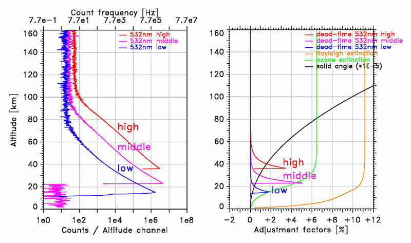
On this page we show how to calculate a night-mean temperature profile from the lidar raw data using as an example the measurement from 13/14 February 2005. The first step is to integrate all recorded profiles from 17 UT und 5 UT. In the following only the signal from the visible channels at 532 nm is used because our lidar has been optimized for this wavelength and therefore has the strongest signal at this wavelength. The integrated raw data from the RMR lidar at 532 nm during this night are shown in the left plot in Figure 1.
Derivation of relative air density profiles
The lidar signal at 532 nm is caused by Rayleigh scattering on air molecules and Mie scattering on aerosols. In addition there is a background caused by light from the atmosphere (stars and moon during night, scattered sunlight during daytime) as well as by electronic noise of the detectors and counters. The following effects have to be taken care of when deriving a relative air density profile from the lidar raw data (see adjustment factors in the right plot of Figure 1):
Dead-time
The RMR lidar employs photomultipliers (PMT) and avalanche photodiodes (APD) in the photon counting mode as detectors. They both have a limit for the shortest interval between two successive photons that can be detected separately. If the photons arrive at shorter intervals, the second photon is lost and will not be counted. As photon counting is a statistical Poisson process, this happens occasionally even if the signal is much lower than the maximum count rate of the detectors. If the maximum count rate is exceeded, incoming photons are lost and not counted. This effect scales with the count rate and is therefore given separately for the three channels in the right plot of Figure 1.
Tilted telescopes
When the telescopes are tilted during a measurement, the light path through the atmosphere is increased. As the counting electronics applies constant time bins, the altitude resolution also changes when the telescopes are titled. Both effects are accounted for in the analysis.
Rayleigh extinction
When the emitted laser pulses propagate upwards in the atmosphere and the scattered light downwards to the telescopes, some photons are scattered by air molecules and lost from the beam. This is called Rayleigh extinction and has to be taken care of when deriving the true air density profile (see orange line in the right plot of Figure 1).
Ozone extinction
The stratospheric ozone layer also leads to an extinktion effect, especially at the green wavelength at 532 nm. This is included into the analysis using ozone profiles from an ozone climatology (see green line in the right plot of Figure 1).
Background subtraction
The magnitude of the height-independent background is determined above 120 km separately from the raw data for each channel. It is then subtracted from the raw data profiles at all heights
Solid angle
This is a geometric effect resulting from the different solid angles covered by the telescope aperture for scattering at different altitudes. The correction is quadratic with the distance between telescope and scatterer and is therefore also called z2 correction (black line in the right plot of Figure 1).
Concatenation of the single profiles
Finally the three single profiles from the upper, middle and lower channel at 532 nm are concatenated resulting in a continuous profile from 20 km to 105 km (see left plot in Figure 2). Above the stratospheric aerosol layer (>30 km) this profile is proportional to the air density in the atmosphere.
The further analysis uses this relative air density profile. To determine the true air density, the lidar system constant and the transmission of the lower atmosphere would need to be known. Fortunately this is not needed to calculate the temperature profile as will be shown in the next section.
Calculation of the temperature profile
Assuming hydrostatic equilibrium, the relative air density profiles can be used to calculate temperature profiles in the aerosol-free part of the atmosphere (>30 km). The temperature T at altitude z can be calculated from the air density profile n as follows
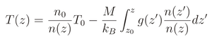
where M is the molecular weight of air, kB is the Boltzmann constant and g is the gravitational acceleration. Additionally the air density n0 at the start height z0 and the start temperature T0 at this height are needed. The latter is taken from the NRLMSISE00 reference atmosphere. Since the equation above only included density ratios, one can directly use the relative density profile derived from the lidar measurements without having to know the system constant of the lidar. Two examples of temperature profiles calculated from RMR lidar measurements are shown in Figure 3. For comparison the figure also includes temperature profiles from measurements with a meteorological rocket and a radiosonde as well as from ECMWF analyses. It shows that these different methods yield similar temperature profiles. The reason for the observed differences is the different temporal and vertical resolution of the different instruments. The ECMWF analyses show large differences at the upper border of the model. They have been investigated in more detail in the comparison of RMR lidar measurements with ECMWF analyses.
Raw data
Density and temperature

Figure 2: Example of a night measurement from 13/14 February 2005 17 UT–5 UT. Left panel: Concatenated profile of the relative air density between 20 km und 105 km. Right panel: Calculated temperature profile for this night (red) with statistical uncertainty (gray), differences in the temperature profile when changing the start temperature by ±20 K (violet) and mean temperature profile from the NRLMSISE00 reference atmosphere (black dashed line).
Temperature comparison
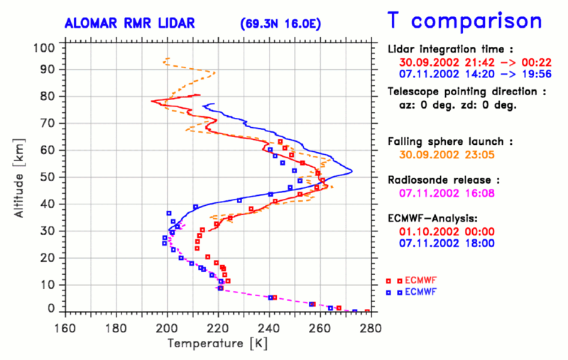
Figure 3: Two examples of temperature profiles from RMR lidar measurements on 30/31 September 2002 and 7 November 2002 (solid red and blue line). For comparison the temperature profile from a measurement with a meteorological rocket (falling sphere, orange dashed line) and a radiosonde (violet dashed line) are shown. Additionally the corresponding temperature profiles from the operational ECMWF analyses are included (red and blue squares).
